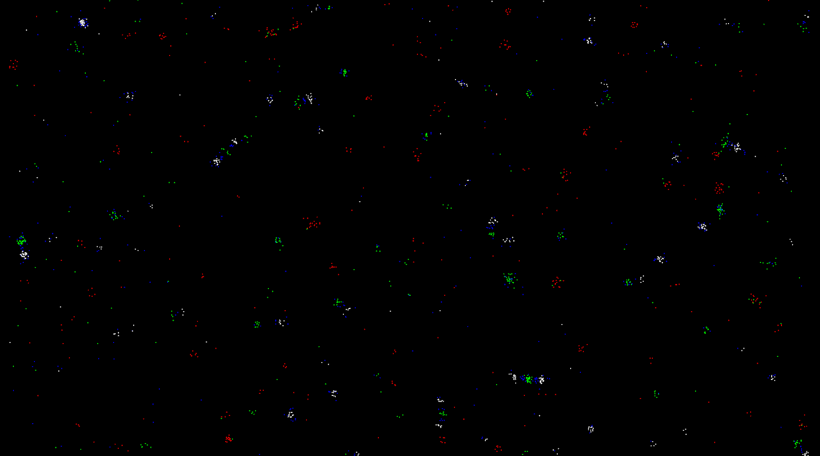
Introduction

Particle Life projects are quite common simulations for programmers interested in physics simulation, optimization, and emergence. I became interested in particle life after seeing videos on youtube (some linked below). I was fascinated by its simplicity, and how something came out of nothing. I used the Unity Game Engine to make this project. I will not go into the code. A github repository will be posted for the code to be used or modified, but I want to make this article about the general algorithm and my experience. The reason this emergent behaviour happens is because of the ignoring of actual physics. Particles create energy out of nothing, they also have asymmetrical attractions. For example particle A is attracted to B, but B is repulsed or not affected by A, and if it were affected by A it would be of different magnitude. This asymmetry leads to more complex behaviour. Yet, how do you find these attractions?

Attraction Matrix and Basic Force Calculation

At the beginning of the simulation certain attraction values are selected for each relation between particle types (including particles of the same type). The attraction is typically represented as a 2D or compressed 1D matrix, ergo ‘Attraction Matrix’. The compressed 1D matrix has the same data as the 2D matrix, but with only one row. You compress it by putting each row after the other. To illustrate the 2D matrix look at:

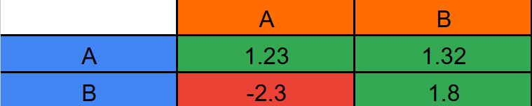
The vertical column is the particle while the horizontal column is the neighbour particle. For any given particle’s force, in a frame for each neighbour particle, you first get the attraction value, multiply that by the unit vector from A to B (magnitude 1 vector with only direction), then you multiply again by a function with a parameter of the closeness between A and B. The way to check if a particle is close enough to another particle to have an effect on velocity is by defining a threshold (affect radius) for them to affect. This can be illustrated as a circle around each particle. If you let 'R' be 'affect radius', and 'M' be the magnitude of the vector from A to B then the closeness, or distance, between particles is: \[ Distance = R - M \] Magnitude is defined with the distance function. Let ‘A’ be the position vector of A, let ‘B’ do the same for B, and let ‘M’ be magnitude. The magnitude is calculated as: \[ M = \sqrt{(A_x-B_x)^2 + (A_y-B_y)^2} \] Each one of these calculations is the main part of the force calculation that happens each frame. The function with a parameter of closeness seems a bit counter intuitive, though. Why can’t you just multiply by the closeness? The explanation is below.

Closeness Function

The reason you should add a closeness function is because it causes more complex behaviour. For example, as suggested earlier, I could replace the closeness function by the actual closeness. But this would only result in a simple linear relationship (it would just be a line). On the other hand, if I used a curved function with dips and bumps I would have local extremes where particles could stay in. The function I used is called the Lennnard-Jones potential, but I modified it with a sine function.

\[ c = 1.5 \] \[ b = 1 \] \[ a = b * c^6 \] \[ f(x) = \left(\frac{a}{x^{12}}\right)-\left(\frac{b}{x^{6}}\right)\ +\ .25\sin x \] Though I don’t know much about the actual physics of the Lennard-Jones potential, I initially used it because of its popularity in the real-world sciences for modeling particle behaviour. It makes particles repulse up close, attract at a moderate distance, and not affect each other from far away. I then added the sine function to it to make more local extremes and to make the attraction not dip off too much at the end. The periodicity of the sine function combined with the base of the Lennard-Jones potential makes artificial particles behave like real world particles while also acting a bit different, for my preference. You could obviously switch this function up if you want to, I actually recommend that.

Additional Aspects

In the pursuit of a more perfect simulation, some changes from typical particle life simulations had to happen. I clamped (made it max out at) the magnitude of the velocity vectors of each particle, to prevent excessive velocity values. I also damped (lowered by a small factor) the velocity for the same purpose. A small random vector was added to the velocity each frame to prevent everything from just not moving. Most importantly, I added a file system to store attraction matrix data for simulation instances that I wanted to see again. The files are in a binary format. The format is as follows:

1. A byte that gives the amount of particle types
2. 3 bytes for each particle type that are RGB colour values of the particles 
respectively.
3. Bytes in the amount of the square of the particle types. These are the attraction 
values. If you let ‘p’ = the amount of particle types Its [0,0], [0,1], ...,[0,p-1],
[1,p-1], ...,[p-1,p-1]

Optimization

For starters, this program is very computationally heavy, because you check each particle for, each particle, each frame. In code, this would be a double-nested for loop with both loops of the same max index, of particle amount. The time complexity of this would be N^2. To fix this, you can do something called spatial partitioning. Spatial partitioning basically makes a grid of square cells, each cell contains a list of particles (more specifically the particle indices). Each cell has a length and width of the particle effect radius. When you calculate forces you first look at one particle, then check and calculate for all neighbouring particles in the same cell and cells nearby. To clarify if you have a particle to apply force to, you look at the cardinal directions, the diagonals, and the same grid cell as the particle. Think of a king in chess, that can move or stay put. This spatial partitioning, grid cell method approaches a time complexity of N, or linear. It can be a lot slower though if you have a bunch of densely packed particles. This is still way faster than N^2. To illustrate the difference, if you had 100 particles: \[ N = 100 \] \[ N^2 = 10,000 \] Afterwards, minor non-algorithm based optimizations can further improve performance. Three things come to mind:

1. Reusing calculations
2. Optimizing powers
3. Taylor Series for sine

Don’t calculate the same thing twice. Instead, store it in a variable and use it. The basic power function in programming languages is not as fast as just doing multiplication. For example, syntax may change by language and framework, but with x as the base and y, which is an integer, as the exponent you should just multiply x times itself y times. The reason this is faster is because the built in power function also generalizes to decimal values, in the exponent, which makes it so the computer has to do a logarithm which is hard for performance (sometimes the language changes if the exponent is an integer). ‘Taylor Series for Sine’ approximates the sine of x. Powers are used in this so you should do the power simplification from earlier.

Conclusion

Finally, after this simple explanation of the ‘Particle Life’ simulation I hope you will understand why I believe it is so beautiful. Something out of nothing, and the very notion of emergence, are fascinations of mine. Life began in similar fashion. Structure from disorder. Complexity from simple rules. Life and Particle Life are similar in this way. I loved seeing the structures. Bug-like replaceable limbs, tendrils like squids, orbits like atoms. The way two objects of similar structures explode and/or sometimes combine into a creature of same or different structure. The way particles that repulse everything lead to a grid like pattern. The way the same structures form again and again in the same simulation instance. How, the start of a simulation can be chaotic but can end up as ordered. I loved it. I hope you will too.

Links

    
How Particle Life emerges from simplicity

Simulating Particle Life

I didn't watch this channel much, but he talks a lot about particle life.
Programming Chaos